Differential Privacy for Privacy-Preserving Data Analyses
Published:
Calculating summary statistics, such as a count of data points, a sum, or an average of values within a dataset cannot be too bad from a privacy perspective, right? These statistics are calculated over a whole dataset at the same time and not on a specific individual, so what could go wrong? In today’s blog post I am going to show you how summary statistics can disclose individual privacy and how the risk can be mitigated with a mathematical framework called Differential Privacy (DP) [1] that formulates privacy guarantees for data analyses methods. For a start, imagine you have a medical dataset that contains 100 data points about diabetes and non-diabetes patients. Since such medical data is highly sensitive, you need to be sure that none of the individuals will suffer any privacy b reach while performing any kind of analysis on them. Bearing that in mind you want to calculate the percentage of each group. Yet, already this simple analysis is not as harmless as it seems when it comes to privacy.
Intuition
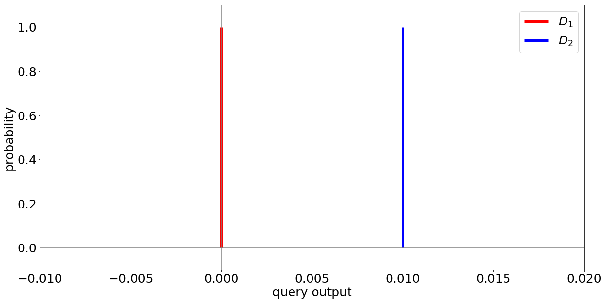
Suppose you start with a patient dataset $D_1$ that contains 100 data points about healthy patients. Then, you replace exactly one of the data points with a data point $x$ of an individual who has diabetes. Let’s call this new dataset $D_2$. $D_1$ and $D_2$ are identical for the 99 other data points, but differ in that one data point $x$ that you’ve replaced. When you calculate the percentage of diabetes patients on both datasets now, you will observe the value 0.0 on $D_1$ and 0.01 on $D_2$.
This difference between the results over the two datasets allows you to learn that individual $x$ has diabetes. Once somebody knows the original dataset and the new one, she can reliably the health status of the added or exchanged individual. Hence, your analysis method cannot be considered privacy-preserving. If you want to read a more thorough explanation of this intuition and notation, you could check out Chapter 3 in my Master Thesis.
This is where DP comes into play. It addresses the goal of learning nothing about an individual while learning useful information about a whole population or dataset. Loosely formulated, DP expresses the following:
Given two datasets that differ in exactly one data point: In order to preserve privacy, the probability for any outcome of your analysis should be roughly the same over both datasets.
Obviously, the average calculation from the previous example does not meet this requirement because if $x$ is a diabetes patient, the probability for the result 0.01 is 100% on $D_2$ but 0% on $D_1$ (because $D_1$ yields the result 0.00 with a 100% probability).
This suggests that deterministic analysis methods (i.e., methods, that on the same data always yield the same results) cannot achieve DP. Instead, what we need to do to protect the individual’s privacy, is to add a controlled amount of probabilistic noise to the results of our analysis. That is, we need a probabilistic analysis. This noise, which can be drawn from a mathematical distribution, such as the Laplace distribution, can dissimulate the difference between the results on both datasets.
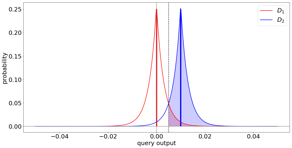
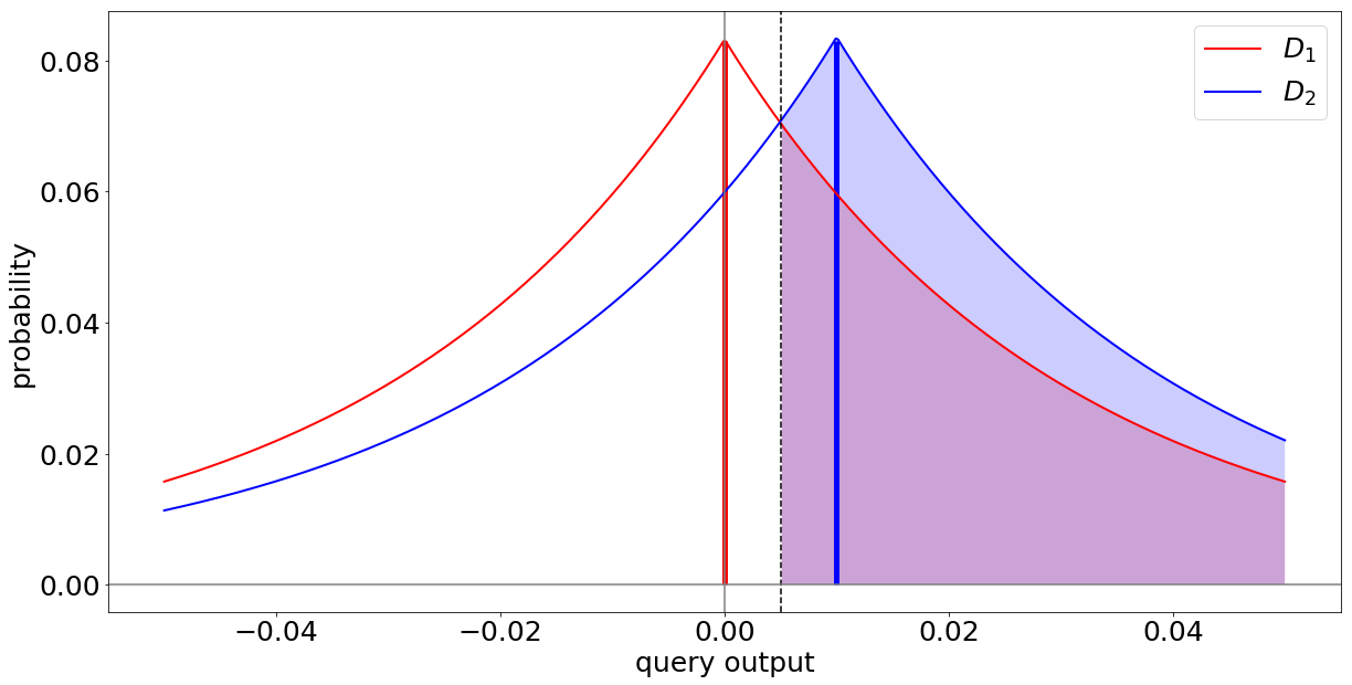
What we see is that depending on the scale of the noise added, the areas below the graphs overlap more. This means that the distribution of results on $D_1$ and $D_2$ get and learning private information about $x$ becomes more difficult.
Definition
This intuition leads to the following definition of DP:
A randomized algorithm $\mathcal{K}$ with domain $\mathbb{N}^{| \mathcal{X}| }$ gives $\epsilon$-DP, if for all neighboring databases $ D_1, D_2 \in \mathbb{N}^{| \mathcal{X}| }$ and all $ S \subseteq Image(\mathcal{K}) $
Definition 1: $\Pr[\mathcal{K}(D_1)\in S] \leq e^\epsilon \cdot \Pr[\mathcal{K}(D_2)\in S] $
To understand the definition, let’s look into its different parts. The randomized algorithm in our example would be the noisy average function. Neighboring data bases refer to databases that only differ in one data point, in our example in $x$.
The definition states that the probability to obtain any specific analysis results on $D_1$ should be roughly the same as obtaining that same result on $D_2$. The roughly the same is expressed by the factor $e^\epsilon$. Alternative formulations refer to $1+\epsilon$, which is a bit more intuitive as it explicitly states that both analysis results should be similar within a factor close to one. However, $e^\epsilon$ has nicer mathematical properties when calculating, for example, with the Laplace distribution.
There also exists a relaxation for $\epsilon$-DP, called $(\epsilon, \delta)$-DP. It is similar to the equation above, but includes a small constant $\delta$ into the formula.
Definition 2: $\Pr[\mathcal{K}(D_1)\in S] \leq e^\epsilon \cdot \Pr[\mathcal{K}(D_2)\in S] + \delta$
The constant $\delta$ can be interpreted as the amount of times that the noisy algorithm is allowed to violate the inequality between the probabilities. Literature usually suggests choosing delta as 1 divided by the number of data samples that you are working with.
Now that you know about the concept of DP, you will be ready for its application in the context of ML that I am going to present next week. If you have questions, comments or remarks, feel free to reach out to me.
Further Reading
[1] Dwork, Cynthia, and Aaron Roth. “The algorithmic foundations of differential privacy.” Foundations and Trends in Theoretical Computer Science 9, no. 3-4 (2014): 211-407.